Calculate the complete route
Include the truck base, loaded legs, unloading points and deadhead movement so all kilometres that consume resources are counted.

Calculate what a European truck trip costs internally before adding margin. Combine loaded and empty distance, country kilometre rates, fuel, tolls, driver time, ferries and other fixed expenses to estimate break-even freight cost.
Freight cost is the economic cost of performing the transport. Keeping it separate from the selling price makes break-even and profit easier to understand.
Include the truck base, loaded legs, unloading points and deadhead movement so all kilometres that consume resources are counted.
Apply country rates, fuel, toll estimates, driver and time cost plus ferries or other route-specific expenses.
Use the internal total and cost per kilometre to understand the minimum economics before commercial uplift is applied.
Internal freight cost = distance cost + fuel + tolls + driver and time cost + route-specific fixed expenses
A transparent calculation keeps each cost driver visible so the dispatcher can see why a route became more or less expensive.
Apply your own kilometre rates to loaded and empty route segments, including country-specific assumptions.
Include the fuel surcharge or operating assumptions used by the selected fleet profile.
Add estimated truck road charges by route country and replace the estimate when a better figure is available.
Account for the economic impact of driving time, pauses, daily rests and elapsed transport time when used by your cost model.
Add ferries, tunnel reservations, handling, parking or other known costs not already contained in the kilometre rate.
Divide the complete internal cost by the complete planned distance to compare route economics on a common basis.
Assume the complete truck movement is 800 km including 75 km of empty positioning. Distance cost, tolls, time cost and route-specific expenses are added to determine the internal freight cost.
Commercial margin is intentionally excluded from the internal total so break-even remains visible.
| Internal cost component | Example amount |
|---|---|
| Distance and fuel cost | €820.00 |
| Estimated tolls | €140.00 |
| Driver and time cost | €95.00 |
| Fixed route expenses | €45.00 |
| Internal freight cost | €1,100.00 |
| Break-even cost per kilometre | €1.38/km |
Illustrative example only. Use your own operating rates, vehicle assumptions and confirmed route charges.
Know the internal route cost before margin changes the number presented to the customer.
Include empty positioning and all operational legs instead of evaluating only loaded kilometres.
Turn total trip economics into a comparable break-even cost per kilometre.
Apply markup only after the internal cost is known, reducing the risk of quoting below the intended margin.
Freight cost is the internal economic cost of performing a transport movement, including the route and operating expenses required to complete it.
No. Freight cost describes the internal expense. Freight price is the selling amount charged to the customer after commercial margin or uplift is applied.
Yes for a complete operating-cost view. Empty kilometres still consume truck capacity, fuel, driver time and other resources.
Yes. LogicCalc can relate complete trip economics to the complete planned route distance so internal cost per kilometre can be reviewed.
This is a real LogicCalc workspace view. Use your own route, cargo, fleet and commercial settings for the actual calculation.
Open LogicCalc →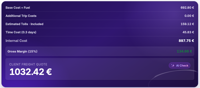
Freight cost is the economic cost of performing the transport. Keeping it separate from the selling price makes break-even and profit easier to understand.
Model what the truck costs to operate over a year before reducing that cost to a route price. Fixed annual expenses and kilometre-driven costs are kept separate so the real cost structure remains visible.
Use this model for fleet economics and budgeting. It answers what the vehicle costs to run, not what one customer should be charged for one shipment.
Enter costs that exist even when the truck is standing still: driver employment, lease or finance, insurance, vehicle tax, depreciation and other recurring annual items.
Convert fuel, AdBlue, maintenance and tyres into kilometre-driven costs using the expected consumption, prices and service assumptions.
Use a realistic annual mileage so fixed costs are not divided by an impossible utilisation level. LogicCalc combines fixed and variable sides into annual cost and operating cost per kilometre.
A truck running 120,000 km per year spreads annual fixed costs across those kilometres, then adds fuel, AdBlue, maintenance and tyres per kilometre. LogicCalc combines both sides into one operating-cost rate before route pricing.
An annual cost model is only as good as the utilisation and cost assumptions behind it.
Fixed costs are incurred mainly with time or ownership, such as lease, insurance and driver employment. Variable costs move mainly with kilometres, such as fuel, AdBlue, maintenance and tyres.
Annual mileage determines how many kilometres carry the fixed-cost burden. If the truck runs fewer kilometres, the fixed cost per kilometre rises even if the annual invoices themselves do not change.
The operating-cost calculator exposes the full annual model and its fixed-versus-variable structure. Cost per kilometre is the unit-rate view produced from that model and is more convenient for route costing.
No. Operating cost is an internal cost baseline. A customer rate may also need empty-mileage recovery, tolls, route-specific charges, commercial margin and market considerations.
Reduce the truck cost model to one internal €/km baseline while keeping the components visible. Fuel, other kilometre-driven costs and the kilometre share of annual fixed expenses should not be mixed into an unexplained single number.
Use cost per kilometre as an internal unit-cost baseline for route economics, benchmarking and rate decisions — not as an automatic customer price.
Translate litres per 100 km and the diesel price into a fuel cost per kilometre. For example, 32 L/100 km at €1.50/L equals €0.48/km before any other cost is added.
Add AdBlue, maintenance, tyres and other kilometre-driven expenses so fuel is not mistaken for the full running cost.
Spread annual driver and vehicle fixed costs across realistic annual mileage, then combine them with variable cost to obtain the internal cost per total kilometre.
With 32 L/100 km at €1.50/L, fuel alone costs €0.48/km. LogicCalc then adds AdBlue, maintenance, tyres and the per-kilometre share of annual fixed costs to show the real operating cost.
A neat €/km number can be misleading if the annual mileage or cost components behind it are incomplete.
No. Fuel is only one variable component. The real truck cost per kilometre can also include AdBlue, maintenance, tyres, driver cost, lease, insurance, tax, depreciation and other fixed expenses.
Yes if the purpose is to estimate the full internal operating cost. Fixed annual costs need to be allocated across realistic annual kilometres so every kilometre carries its share of the vehicle and driver cost base.
The internal cost-per-total-kilometre baseline should reflect every kilometre the truck actually runs. To convert that into the minimum revenue needed per loaded kilometre, use the break-even rate calculation with the empty-mileage share.
Usually not. It is an internal cost baseline. A sell rate may also need empty-mileage recovery, tolls, trip-specific charges, margin and the commercial conditions of the job.
Translate internal cost per total kilometre into the minimum revenue required from loaded kilometres. Empty running matters because the paid kilometres must recover the cost of kilometres that generate no freight revenue.
Use the break-even rate when deciding whether a loaded-kilometre offer actually recovers the truck’s total running, including deadhead.
Use the full internal truck cost per kilometre, not only fuel. Every actual kilometre creates cost whether the vehicle is loaded or empty.
Convert the empty-mileage percentage into the share of kilometres that can earn freight revenue. Divide the cost per total kilometre by that loaded share to find the break-even rate per loaded kilometre.
Break-even only covers the modeled cost base. If a commercial target is required, apply the desired margin or uplift after the cost-covering loaded rate is known.
If a truck costs €1.10 per total kilometre and 15% of annual kilometres are empty, the break-even rate rises to about €1.29 per loaded kilometre. A target margin can then be applied on top.
Break-even is a planning threshold, not a promise that a particular load will be profitable after every real-world cost is known.
Because loaded kilometres must pay for both loaded and empty running. When some kilometres earn no freight revenue, the cost of those kilometres has to be recovered from the smaller loaded share.
A simple planning model divides internal cost per total kilometre by the loaded-kilometre share. At €1.10/km total cost and 15% empty mileage, the loaded share is 85%, giving about €1.29 per loaded kilometre before target profit.
No. Break-even is the modeled cost-covering threshold. A target selling rate may be higher to provide profit and cover risk, route-specific charges or commercial conditions.
The loaded share becomes smaller, so each revenue kilometre must recover more total truck cost. The break-even loaded rate therefore rises even if the underlying cost per total kilometre does not change.
LogicCalc creates a separate positioning leg between the configured truck base and the first route point. That leg is shown as empty deadhead and is included in route distance and distance-based cost.
Add the vehicle starting location in Fleet Profile settings. This becomes the origin of the optional empty positioning route.
Add the first loading point and the remaining loading, unloading or intermediate stops.
LogicCalc adds deadhead distance to the loaded route and includes its country-rate cost, fuel use and effect on the final price.
Total planned distance = empty positioning distance + sum of all loaded and intermediate route legs
The financial effect of deadhead depends on the distance from the base, the countries crossed, configured kilometre rates and how the positioning run affects fuel and transit time.
The saved base location determines where the empty positioning route begins.
The first active route point becomes the destination of the empty leg.
LogicCalc calculates a real road leg instead of using straight-line distance.
Each country segment of the empty route can use its own configured euro-per-kilometre rate.
Fuel reporting can distinguish the positioning run and apply the empty-vehicle consumption factor.
Deadhead cost becomes part of internal route economics before margin and client price are calculated.
Assume the truck is based 145 km from the first loading point. The loaded route after pickup is 690 km, giving a complete planned distance of 835 km.
In this simplified example, the empty and loaded legs use different average kilometre rates. A 10% fuel surcharge is then calculated from the combined distance-based route cost.
| Route component | Example result |
|---|---|
| Empty positioning distance | 145 km |
| Loaded route distance | 690 km |
| Total planned distance | 835 km |
| Empty positioning cost | €181.25 |
| Loaded route cost | €931.50 |
| Fuel surcharge (10%) | €111.28 |
| Base route cost plus fuel | €1,224.03 |
Illustrative example only. Actual results depend on the road route, country split, configured rates, fuel settings and vehicle profile.
Empty mileage, deadhead or positioning distance is the distance a truck travels without the transport cargo, for example from its base to the first loading point.
When a truck starting base is entered, LogicCalc builds a separate road route from that base to the first route point and stores it as the positioning leg.
Yes. The positioning distance is added to the sum of the remaining route legs for route KPIs, transit planning and cost calculation.
Yes. The deadhead route has its own country breakdown, and the configured rate for each country can be used to calculate its cost.
Because the deadhead distance-based cost is included in the base route calculation, it also affects a percentage-based fuel surcharge.
That is a commercial decision. LogicCalc shows the cost so the dispatcher can decide how much of it must be recovered in the quoted price.
Estimate how much fuel a truck is likely to use on a calculated route from route distance, the active truck consumption profile and payload. The result is a planning estimate in litres, not a measurement from the vehicle.
route distance, truck fuel-consumption profile and payload
estimated litres of fuel and payload-adjusted consumption
Use the road distance of the calculated trip rather than straight-line distance. Fuel demand scales with the kilometres the truck is expected to drive.
Apply the reference fuel-consumption setting of the active truck profile together with the current payload information used by LogicCalc.
Use the resulting fuel quantity as a planning input for trip economics and CO₂, and update the profile when the truck or load changes.
A 600 km route with a reference consumption of 30 L/100 km starts from about 180 L before payload adjustments. LogicCalc can adjust the estimate according to the active truck profile and load.
A 600 km route with a reference consumption of 30 L/100 km starts from about 180 L before payload adjustments. LogicCalc can adjust the estimate according to the active truck profile and load.
Keep the route, truck profile and payload aligned with the actual job; otherwise a precise-looking litre result can still be based on the wrong assumptions.
The page uses calculated route distance together with the active truck fuel-consumption profile and payload information.
No. It is a planning estimate. Actual litres can differ because the executed trip and real conditions may differ from the calculation inputs.
The page is designed to adjust the estimate using the current load together with the truck profile, so the same route can produce a different estimate for a different payload.
Fuel consumption estimates litres used on a trip. Cost per kilometre combines fuel with other variable and fixed operating costs to produce an internal €/km baseline.
Estimate road freight CO₂ emissions from route distance and vehicle assumptions, compare transport scenarios and include an ESG result with LogicCalc.
A simplified route estimate multiplies vehicle activity by an emission factor. The usefulness of the result depends on consistent distance data and assumptions that match the vehicle and reporting purpose.
Build the complete route, including relevant empty positioning, so the estimate uses the movement actually planned.
Use the factor associated with the selected vehicle or the company reporting method.
Compare route scenarios and include the estimated emissions in the route summary or customer-facing PDF.
Estimated CO₂e = route distance × selected vehicle emission factor
Vehicle technology, fuel, load, distance, empty running, road conditions and the chosen reporting boundary can all affect the final emissions figure.
Use the calculated road distance for the complete movement rather than straight-line distance.
Include relevant deadhead travel when the reporting boundary covers the full vehicle movement.
Select assumptions that reflect the truck, fuel and operating profile used for the route.
Apply a consistent factor expressed per vehicle kilometre or another clearly defined reporting unit.
Keep weight, loading metres and utilisation visible because they help explain the efficiency of the movement.
Present the estimate with the calculation scope and assumptions instead of showing an unexplained CO₂ number.
Assume the complete vehicle route is 780 kilometres and the selected planning factor is 0.80 kilograms of CO₂e per vehicle kilometre.
The simplified result is 624 kilograms of CO₂e. A different vehicle, fuel, load factor or reporting standard can produce a different figure for the same route.
| Emissions input | Example value |
|---|---|
| Complete route distance | 780 km |
| Planning emission factor | 0.80 kg CO₂e/km |
| Loaded and empty movement | Included |
| Estimated route emissions | 624 kg CO₂e |
Illustrative estimate only. Use approved company or reporting-standard factors when the result is required for formal disclosure.
See how distance, empty positioning and vehicle assumptions change the estimated emissions.
Calculate from the same route used for cost and time planning instead of entering an unrelated distance.
Include a transparent estimate and its assumptions in the route summary when emissions information is requested.
Review CO₂, price, transit time, cargo space and vehicle utilisation as connected planning results.
CO₂e means carbon dioxide equivalent. It expresses different greenhouse gases as a comparable amount of carbon dioxide based on their warming effect.
Distance is a major input, but the emission factor should reflect the vehicle, fuel, operation and reporting method used for the estimate.
Include them when the reporting boundary covers the complete vehicle movement. Excluding deadhead travel can understate route activity.
Only when the methodology, emission factors, data quality and reporting boundary satisfy the relevant company or external standard. A planning estimate alone may not be sufficient.
This is a real LogicCalc workspace view. Use your own route, cargo, fleet and commercial settings for the actual calculation.
Open LogicCalc →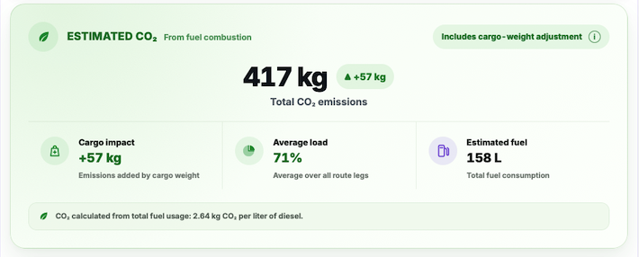
CO₂ results are estimates. Formal reporting may require approved well-to-wheel or tank-to-wheel factors, fuel data, load allocation, empty-running rules and a documented methodology.
Explore route planning, transport pricing, cargo, driver-time and sustainability tools in one connected workspace.
Calculate the complete route economics first, then use the internal result as the foundation for freight pricing and profitability decisions.
Freight cost results are planning estimates based on configured and entered values. Verify actual fuel, toll, wage, ferry, maintenance, vehicle and contractual costs used by your business.